1. Euler's method if * = f(t,y)
so, y(i+1) = y(i) + f(ti,yi)h ; h is step size
Problem :: dx/dt = -x +10 = f(ti,xi)
x(i+1) = x(i) + f(ti,xi)*h
พิมสูตรใส่ m-file
clear, clc
%problem
dx = @(x) - x +10;
t(1) = 0; %t ที่เวลาต่าง
x(1)= 1; %initial value
h = 1; %step size
time = 10;
n = time/h;
% make for loop
for i = 1:1:n %start from 1: increase 1 : to n
t(i+1) = t(i) + h;
x(i+1) = x(i) + dx(x(i))*h;
end
plot(t,x) %วาดกราฟ
เมื่อ RUN แล้ว กราฟจะได้กราฟขึ้นมา
จะได้ คำตอบ x ในหน้า command window
>> x
x =
1 10 10 10 10 10 10 10 10 10 10
การพล็อต 2 กราฟ
clear, clc
%problem
dx = @(x) - x +10;
t(1) = 0; %t ที่เวลาต่าง
x(1)= 1; %initial value
h = 1; %step size
time = 10;
n = time/h;
% make for loop
for i = 1:1:n %start from 1: increase 1 : to n
t(i+1) = t(i) + h;
x(i+1) = x(i) + dx(x(i))*h;
end
plot(t,x, 'b') %ให้แสดงกราฟเป็นเส้นทึบ
h = 0.01;
n = time/h;
% make for loop
for i = 1:1:n %start from 1: increase 1 : to n
t(i+1) = t(i) + h;
x(i+1) = x(i) + dx(x(i))*h;
end
hold on %ให้กราฟเดิมยังอยู่
plot(t,x, 'r--') %r-- ให้แสดงกราฟเป็นเส้นประสีแดง
การทำ ให้เป็น function ไว้เรียกใช้
function Euler
function [t,x] = fEuler(dx,x0,time,h)
t(1) = 0;
x(1)= x0;
n = time/h;
% make for loop
for i = 1:1:n %start from 1: increase 1 : to n
t(i+1) = t(i) + h;
x(i+1) = x(i) + dx(x(i))*h;
end
การเรียกใช้ function Euler ที่เราทำไว้
เปิดหน้า M-file ขึ้นมาใหม่ แล้วใส่ปัญหาของเราไป
clear, clc
dx = @(x) - x +10;
x0= 1; %initial value
h = 1; %step size
time = 10;
[t,x] = fEuler(dx,x0,time,h);
plot(t,x)
กด RUN แล้วลอง หาX ในหน้า command window
จะได้ คำตอบ x ในหน้า command window
>> x
x =
1 10 10 10 10 10 10 10 10 10 10
สร้างสมการจาก system


problem A
สร้างใน M-file
clear,clc
w1 = 500;
w2 = 200;
x1 = 0.4;
x2 =0.75;
model_ss = @(x) w1*(x1-x)+ w2*(x2-x);
[x, fval,exitflag] = fzero(model_ss,1);
%1 equation, 1 variable :: must be use fzero to solve
%check exitflag
***note 1 สมการ 1ตัวแปร ใช้ fzero ในการคำนวณ
แต่ถ้าเป็น หลายสมการ หลายตัวแปร จะใช้ fsolve แทนนะจ๊ะ ***
เชคคำตอบที่หน้าคอมมานวินโดว์
>> x
x =
0.5000
>> [x, fval,exitflag]
ans =
0.5000 0.0000 1.0000
Problem B
ใน M-File
%problem b : w1 changes from 500 to 400
w1 = 400;
w2 = 200;
x1 = 0.4;
x2 =0.75;
model_ss = @(x) w1*(x1-x)+ w2*(x2-x);
x0 = 0.5;
[x, fval,exitflag] = fzero(model_ss,x0);
คำตอบใหม่คือ x ลู่เข้าสู่ ...เช็คได้จากหน้า คอมมานวินโดว์
>> x
x =
0.5167
Pb.A และ Pb.B เป็นการคิดที่ steady state
ถ้าไม่เป็น SS ใช้ ODE คำนวณ
การสร้าง ODE
clear, clc
w1 = 400;
w2 = 200;
x1 = 0.4;
x2 =0.75;
model_ss = @(x) w1*(x1-x)+ w2*(x2-x);
x0 = 0.5;
[x, fval,exitflag] = fzero(model_ss,x0);
v=2;
p=900;
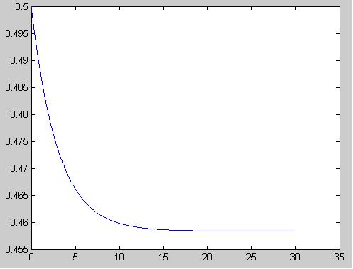
model_dyn = @(x) w1/v/p*(x1-x) + w2/v/p*(x2-x);
time = 30;
h=0.01;
[t,x] = fEuler(model_dyn,0.5,time,h);
plot(t,x)
** คำตอบดูจากกราฟ ว่า มีแนวโน้มถูกต้องหรือไม่ **

Pb. C ใน M-file
%Pb C w2 chenges 200 to 100
clear, clc
w1 = 500;
w2 = 100;
x1 = 0.4;
x2 =0.75;
model_ss = @(x) w1*(x1-x)+ w2*(x2-x);
x0 = 0.5;
[x, fval,exitflag] = fzero(model_ss,x0);
v=2;
p=900;
model_dyn = @(x) w1/v/p*(x1-x) + w2/v/p*(x2-x);
time = 30;
h=0.01;
[t,x] = fEuler(model_dyn,0.5,time,h);
plot(t,x)
จะได้กราฟคำตอบ
Pb.D ใน M-file
%Pb D x1 chenges 0.4 to 0.6
clear, clc
w1 = 500;
w2 = 200;
x1 = 0.6;
x2 =0.75;
model_ss = @(x) w1*(x1-x)+ w2*(x2-x);
x0 = 0.5;
[x, fval,exitflag] = fzero(model_ss,x0);
v=2;
p=900;
model_dyn = @(x) w1/v/p*(x1-x) + w2/v/p*(x2-x);
time = 30;
h=0.01;
[t,x] = fEuler(model_dyn,0.5,time,h);
plot(t,x)
จะได้กราฟคำตอบเป็น

การใช้ model "ode45" หรือ SK model
ใช้โจทย์ Pb.B
สร้าง function ของ dynamic model ขึ้นมาก่อน
function df = fblending_tank(t,x)
%input
w1 = 400;
w2 = 200;
x1 = 0.4;
x2 =0.75;
%parameter
v = 2;
p = 900;
%dynamic model
df = w1/v/p*(x1-x) + w2/v/p*(x2-x);
เปรียบเทียบ ระหว่าง คำตอบที่ได้จาก Euler และ ode45
clear, clc
w1 = 400;
w2 = 200;
x1 = 0.4;
x2 =0.75;
model_ss = @(x) w1*(x1-x)+ w2*(x2-x);
x0 = 0.5;
[xss, fval,exitflag] = fzero(model_ss,x0);
v=2;
p=900;
model_dyn = @(x) w1/v/p*(x1-x) + w2/v/p*(x2-x);
time = 30;
h=0.01;
[t,x] = fEuler(model_dyn,x0,time,h);
plot(t,x,'b')
[t1,x1] = ode45(@fblending_tank,[0 time],0.5);
hold on
plot (t1,x1,'r--')
จะได้กราฟคำตอบ

จะได้ว่ากราฟสองเส้นทับกันพอดี!
check คำตอบที่หน้า คอมมานวินโดว์
>> x
x =.
.
.
.
Column 3001
0.5167
สุดท้าย x ลู่เข้าสู่ค่า 0.5167
Example System 2


*มีหลายสมการ ใช้ fsolve*
At Steady state
สร้าง Function ขึ้นมาก่อน ใน M-file
function df = fTank_heater_ss(x)
h= x(1);
T= x(2);
%inputs
Fi = 300; %cm3/s
Ti = 25; %Oc
Q = 5000; %J
%parameter
Cv = 50;
%A = 100; %cm2
%p = 1; %g/cm3
Cp = 4.184; %J/g.C
df = [Fi - Cv*sqrt(h)
Fi/h*(Ti-T) + Q/h/Cp]; %steady state Model
แก้สมการ โดยใช้ fsolve ใน M-file
clear, clc
x0 = [1 1];
[x, fval,exitflag] = fsolve(@fTank_heater_ss,x0);
%fval is function value at x
จะได้คำตอบในคอมมาานวินโดว์
>> x
x =
36.0000 28.9834
Un_SS
สร้างสมการ ที่ Unsteady state in M-file
function df = fTank_heater_dyn(t,x)
h= x(1);
T= x(2);
%inputs
Fi = 300; %cm3/s
Ti = 25; %Oc
Q = 5000; %J
%parameter
Cv = 50;
A = 100; %cm2
p = 1; %g/cm3
Cp = 4.184; %J/g.C
df = [Fi - Cv*sqrt(h)
Fi/A/p/h*(Ti-T) + Q/A/p/h/Cp]; %Unsteady state Model
แก้สมการ โดยใช้ ode45
clear, clc
x0 = [1 1];
[xss, fval,exitflag] = fsolve(@fTank_heater_ss,x0);
%fval is function value at x
x0 = xss;
[t,x] = ode45(@fTank_heater_dyn,[0 20],x0);
จะได้คำตอบในคอมมานวินโดว์
>> x
x =
36.0191 28.9834
36.0163 28.9834
36.0140 28.9834
36.0120 28.9834 ......
พล็อตกราฟเพื่อดูค่า ใน M-File
clear, clc
x0 = [1 1];
[xss, fval,exitflag] = fsolve(@fTank_heater_ss,x0);
%fval is function value at x
x0 = xss;
[t,x] = ode45(@fTank_heater_dyn,[0 20],x0);
plot(t,x(:,1))
figure
plot(t,x(:,2))
จะได้กราฟ

รูปที่ 1 และ 2 แสดงค่าที่ SS ค่าทีไ่ด้จะเป็นเส้นตรง (ที่เหวียงๆข้างหลัง คือ numerical error)
ลองเปลี่ยนค่า
Fi = 200 ดู
จะได้กราฟ

แสดงลักษณะที่ได้ ^^
เสร็จจ้าาาาา!!!!!
ไม่มีความคิดเห็น:
แสดงความคิดเห็น